Multilayer Neural Networks
Multilayer neural networks contain more than one computational layer.
The perceptron contains an input and output layer, of which the output layer is the only computation-performing layer.
The input layer transmits the data to the output layer, and all computations are completely visible to the user.
Multilayer neural networks contain multiple computational layers;
the additional intermediate layers (between input and output) are referred to as
hidden layers
because the computations performed are not visible to the user.
The specific architecture of multilayer neural networks is referred to as
feed-forward networks,
because successive layers feed into one another in the forward direction from input to output.
The default architecture of feed-forward networks assumes that all nodes in one layer are connected to those of the next layer.
Therefore, the architecture of the neuralnetwork is almost fully defined,
once the number of layers and the number/type of nodes ineach layer have been defined.
The only remaining detail is the loss function that is optimized in the output layer.
Although the perceptron algorithm uses the perceptron criterion, this is not the only choice.
It is extremely common to use softmax outputs with cross-entropyloss for discrete prediction
and linear outputs with squared loss for real-valued prediction.
As in the case of single-layer networks, bias neurons can be used both in the hidden layers and in the output layers.
Examples of multilayer networks with or without the bias neurons are shown in Figure1.11(a) and (b) respectively.
In each case, the neural network contains three layers.
Note that the input layer is often not counted, because it simply transmits the data and no computation is performed in that layer.
If a neural network contains
p1...pk units in each of its k layers, then the (column) vector representations of
these outputs, denoted by ħ
1...ħ
k have dimensionalities p
1...p
k.
Therefore, the numberof units in each layer is referred to as the
dimensionality of that layer.
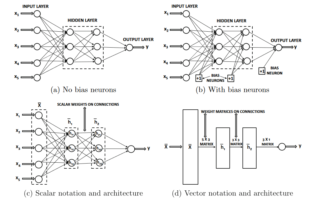
The basic architecture of a feed-forward network with two hidden layers and
a single output layer. Even though each unit contains a single scalar variable, one often represents all units within a single layer
as a single vector unit. Vector units are often represented as rectangles and have connection matrices between them.
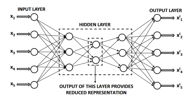
An example of an autoencoder with multiple outputs
The weights of the connections between the input layer and the first hidden layer are contained in a matrix W1 with sized xp1,
whereas the weights between the r
th hiddenlayer and the (r+ 1)
th hidden layer are denoted by the p
r x p
r+1
matrix denoted byW
r.
If the output layer contains
o nodes, then the final matrix W
k+1 is of size p
k x
o.
The d-dimensional input vector x is transformed into the output s using the following recursive equations:
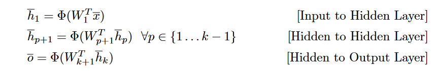
Here, the activation functions like the sigmoid function are applied in element-wise fashion to their vector arguments.
However, some activation functions such as the softmax (which are typically used in the output layers) naturally have vector arguments.
Even though each unit of a neural network contains a single variable, many architectural diagrams combine the units in a single layer
to create a single vector unit, which is represented as a rectangle rather than a circle.
For example, the architectural diagram in Figure1.11(c) (with scalar units) has been transformed to
a vector-based neural architecture in Figure1.11(d)
Note that the connections between the vector units are now matrices.
Furthermore, an implicit assumption in the vector-based neural architecture is that all units in a layer use the
same activation function, which is applied in element-wise fashion to that layer.
This constraint isusually not a problem, because most neural architectures use the same activation function through out
the computational pipeline, with the only deviation caused by the nature of the output layer.
Throughout this neural networks series in this website, neural architectures in which units contain vector variables
will be depicted with rectangular units, where as scalar variables will correspond to circular units.
Note that the aforementioned recurrence equations and vector architectures are valid only for layer-wise feed-forward networks,
and can not always be used for unconventional architectural designs.
It is possible to have all types of unconventional designs in which inputs might be incorporated in intermediate layers,
or the topology might allow connections between non-consecutive layers.
Furthermore, the functions computed at a node may not always be in the form of a combination of a linear function
and an activation. It is possible to have all types of arbitrary computational functions at nodes.
Although a very classical type of architecture is shown in Figure1.11, it is possible to vary on it in many ways,
such as allowing multiple output nodes. These choices are often determined by the goals of the application at hand
(e.g., classification or dimensionality reduction).
A classical example of the dimensionality reduction setting is the auto encoder,which recreates the outputs from the inputs.
Therefore, the number of outputs and inputs is equal, as shown in Figure1.12.
The constricted hidden layer in the middle outputs
the reduced representation of each instance. As a result of this constriction, there is some loss in the representation,
which typically corresponds to the noise in the data.
The outputs of the hidden layers correspond to the reduced representation
of the data. In fact, a shallow variant of this scheme can be shown to be mathematically equivalent to a well-known dimensionality reduction
method known as singular value decomposition.
As we will see in the coming posts,
increasing the depth of the network results in inherently more powerful reductions.
Although a fully connected architecture is able to perform well in many settings, better performance is often achieved by
pruning many of the connections or sharing them in an insightful way.
Typically, these insights are obtained by using a
domain-specific understanding of the data.
A classical example of this type of weight pruning and sharing is that of the convolutional neural network architecture,
in which the architecture is carefully designed in order to conform to the typical properties of image data.
Such an approach minimizes the risk of overfitting by incorporating domain-specific insights (or bias).
As we will see in the coming posts , overfitting is a pervasive problem inneural network design,
so that the network often performs very well on the training data, but it generalizes poorly to unseen test data.
This problem occurs when the number of free parameters, (which is typically equal to the number of weight connections),
is too large compared to the size of the training data.
In such cases, the large number of parameters memorize the specific nuances of the training data,
but fail to recognize the statistically significant patterns for classifying unseen test data.
Clearly, increasing the number of nodes in the neural network tends to encourage overfitting.
Much recent work has been focused both on the architecture of the neural network as well as on the computations performed
within each node in order to minimize overfitting.
Furthermore, the way in which the neural network is trained also has an impact on the quality of the final solution.
Many clever methods, such as pre-training, have been proposed in recent years in order to improve the quality of the learned solution.
This website will explore these advanced training methods in detail.